Conditional formatting allows you to format an excel cell, or cells, in a particular way depending on the data contained in the cell.

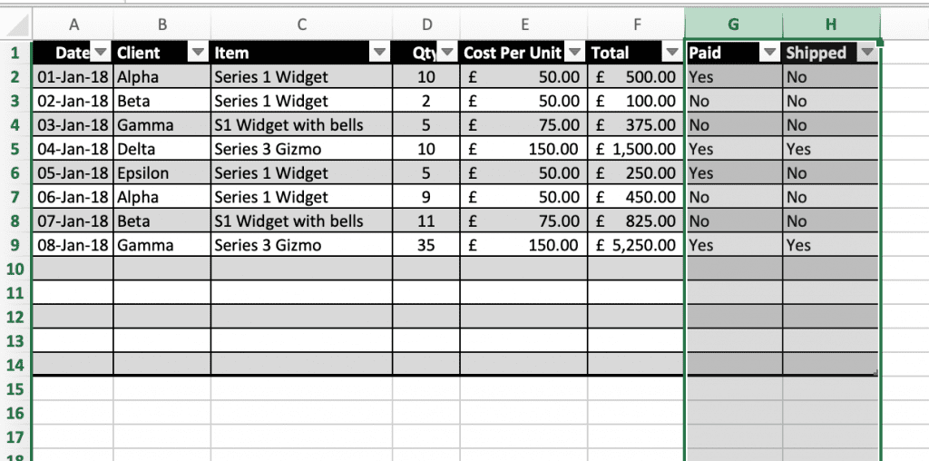
For example, a quick glance of the simple spreadsheet below does not make it obvious which clients have paid or which orders have been shipped.

Formatting each cell would become very time consuming and annoying. So Excel has a very powerful built in tool Called “Conditional Formatting” which can be found in the ribbon tool bar at the top of the excel window.

Within a few clicks it is possible to format text in certain cells or columns to change colour for certain values. In this example we are going to highlight “Yes” as GREEN and no “No” as RED, as shown below…

Step, by step guide…

Step 1, Highlight the columns you would like the conditionally formatted. In this example we are have selected columns G & H

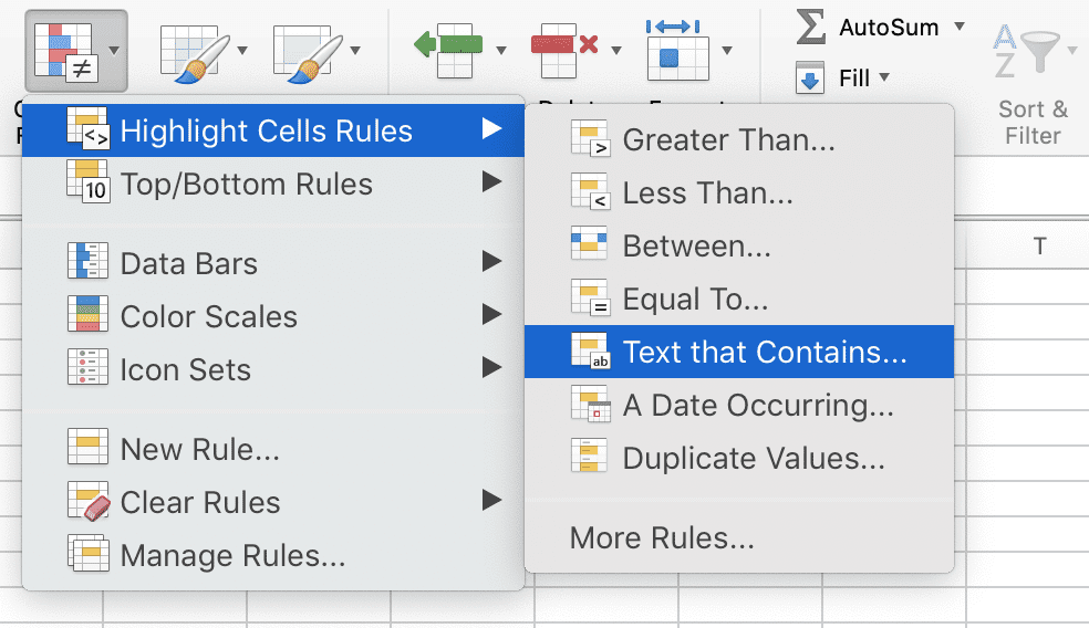
Step 2, Choose, Conditional formatting… Highlighted Cells Rules… Text the Contains… as shown below…

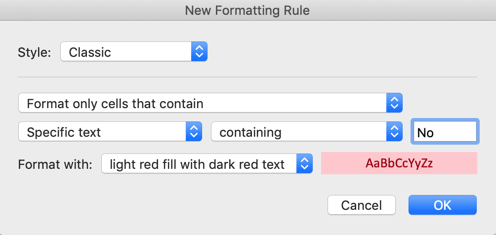
Step 3, Type “No” in the text field and choose “light red fill with dark red text” in the dialogue box. Then Click OK

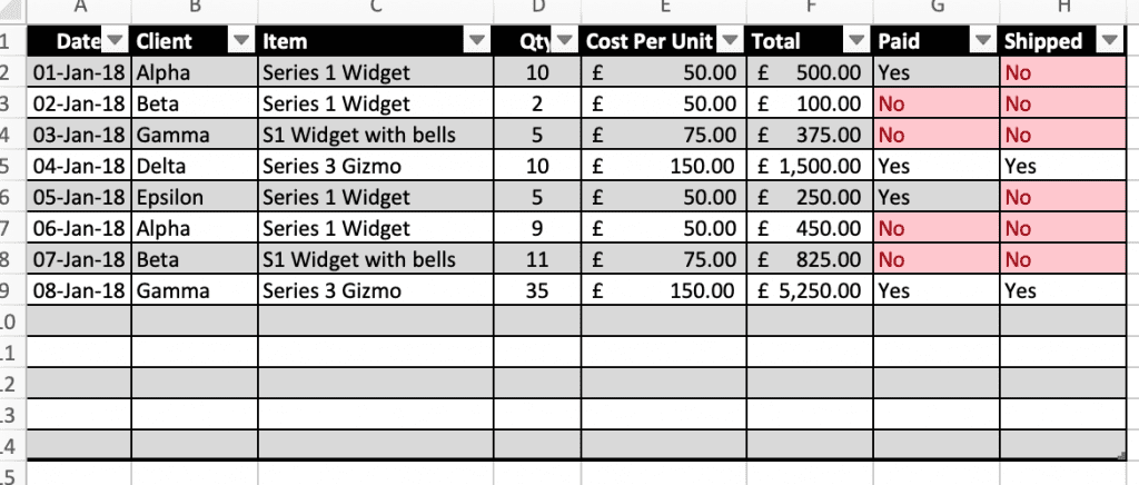
When you click OK the spreadsheet should look like the image below, with all of the “No” cells highlighted in red…

Repeat Steps 1 & 2, and then….

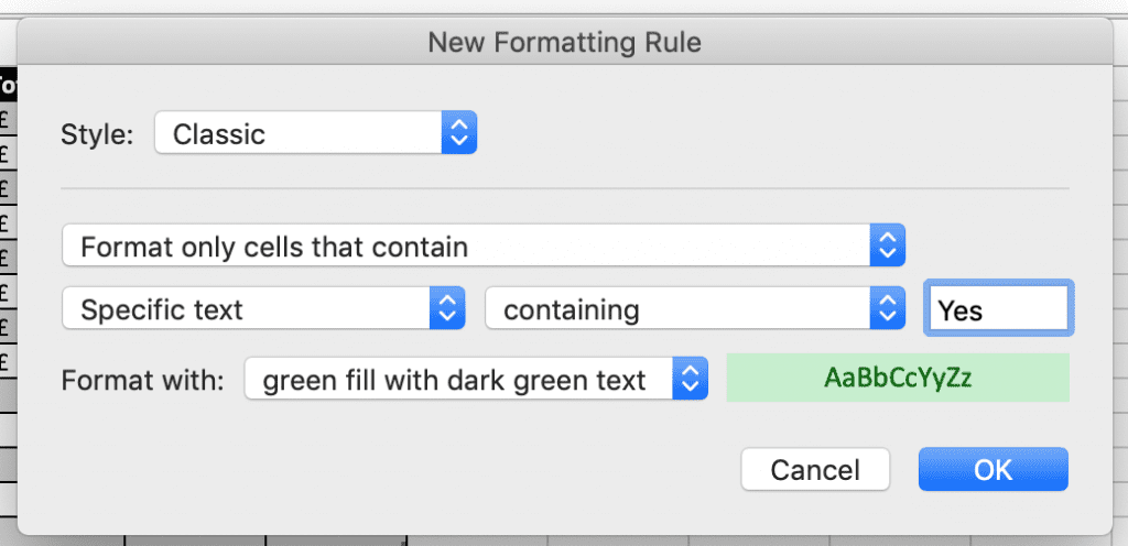
Step 4, Type “Yes” in the text field and choose “green fill with dark green text” in the dialogue box. Then Click OK

If you have completed all of the steps successfully the spreadsheet will now look like this….

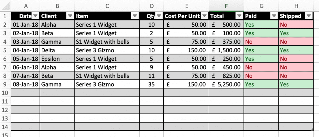
Any time you type either Yes or No in Columns G or H they will automatically be formatted in the styles we have chosen.

Want more Tips?

If you would like to receive hints and tips directly into your inbox, please sign up here…